Does the LTV Forecast Work on Real Data?

Written to a disclosure policy: errors, rankings, biases and coverage are reported as measured; totals, prices and dates finer than a year are withheld, and the two titles are pseudonyms. Every figure traces to a named table, listed at the end.

---

The question

This study is named for cohort lifetime value, and for its first two months every LTV accuracy figure in it came from a synthetic generator. I had built the generator deliberately: it produces free-to-play cohorts with a known ground-truth D365 net LTV, so a forecast made from the first week of a cohort’s life can be scored against the right answer instead of a proxy. That is the argument for synthetic data, and it is a good one.

It is also, I came to realise, the weakest possible place to rest the central claim — because this study’s own cost-per-install result was that synthetic data compresses every model into a narrow band and ranks the wrong one first. If that was true of CPI, why would it not be true of LTV?

Both real warehouses observe cohorts for years. So the question could simply be settled: take a real cohort, pretend only its first w months are known, forecast the rest of its revenue-per-install curve from prior cohorts that were observable at that moment, and compare the implied LTV against what the cohort actually went on to earn. Two titles, scored independently. The decision this serves is the one the whole study exists for: how early can a studio know what a cohort is worth, well enough to change what it spends on the next one?

Why a cohort’s value is harder to observe than it looks

A cohort’s LTV at twelve months is not observable until the cohort is twelve months old. By then the decision it would have informed — whether to keep buying users like these — is eleven months stale. So every usable LTV number is a forecast, and the question is how much of the eventual total is visible from the early months.

The information available at the moment of decision comes from two places. The cohort’s own banked revenue so far — which is certain, and which is the whole of what a “naive” forecast assumes. And the shapes traced by prior cohorts — which tell you how much a cohort of this age typically has left to earn. The standard studio heuristic combines them in one step: multiply banked revenue by the historical ratio of eventual LTV to revenue-at-this-age. A fitted cohort curve is the more elaborate version of the same idea. Whether the elaboration earns its keep was exactly what I did not know.

My approach

Three forecasters, scored on exactly the same cohorts (ltv_validation__ltv_accuracy):

• curve_champion — the study’s selected cohort curve for revenue per install, forecasting the unobserved ages from prior cohorts observable at the origin.
• naive_banked — the cohort earns nothing more than it already has.
• cohort_ratio — banked revenue scaled by prior cohorts’ realised LTV multiple.

The like-for-like scoring is the part I got wrong first. The ratio baseline needs more history to exist at all — a cohort cannot have a realised multiple until some prior cohort has reached the target age — so on a first run it was scored on far fewer, easier cohorts than the curve model and appeared to win comfortably. Restricting every comparison to the cells all three models can predict partly reversed that. Print the cell count next to every score; an unexplained difference in n is the tell.

Then the same task on the synthetic cohorts, forecasting D365 LTV from observation windows measured in days (ltv_validation__ltv_synthetic_reference), so the two worlds can be put side by side.

The assumptions doing the heavy lifting

Prior cohorts are informative about this one. The whole method rests on the newest cohort eventually tracing roughly the shape its predecessors traced. The cohort-quality work says this is systematically a little optimistic — each cohort is slightly worse than the last — and the bias figures below are what that optimism looks like.

Revenue is on the warehouses’ own basis, gross of platform fees. The synthetic study reports LTV net. The comparison between them is like-for-like in method, not in accounting.

Cohorts under a size floor are excluded, because a per-install rate on a tiny cohort is mostly noise. Both titles lose their earliest and latest months this way.

One specification, not a bake-off. This tests the revenue curve the chain work had already selected, so it inherits that choice rather than re-litigating it for the LTV task specifically.

Where reality became inconvenient

The second title cannot adjudicate the two-year result. At a cohort age of twenty-four months, the number of cohorts old enough to score at all on the second title is two from three months observed, five from six, and eleven from twelve. The first title has seventeen to twenty-eight. Two to eleven cohorts cannot separate three models, and the ordering there — where the curve model loses to banked-to-date at every window — should not be reported as a replication failure any more than as a success. I read that row as unmeasured. That will not change until the panel does.

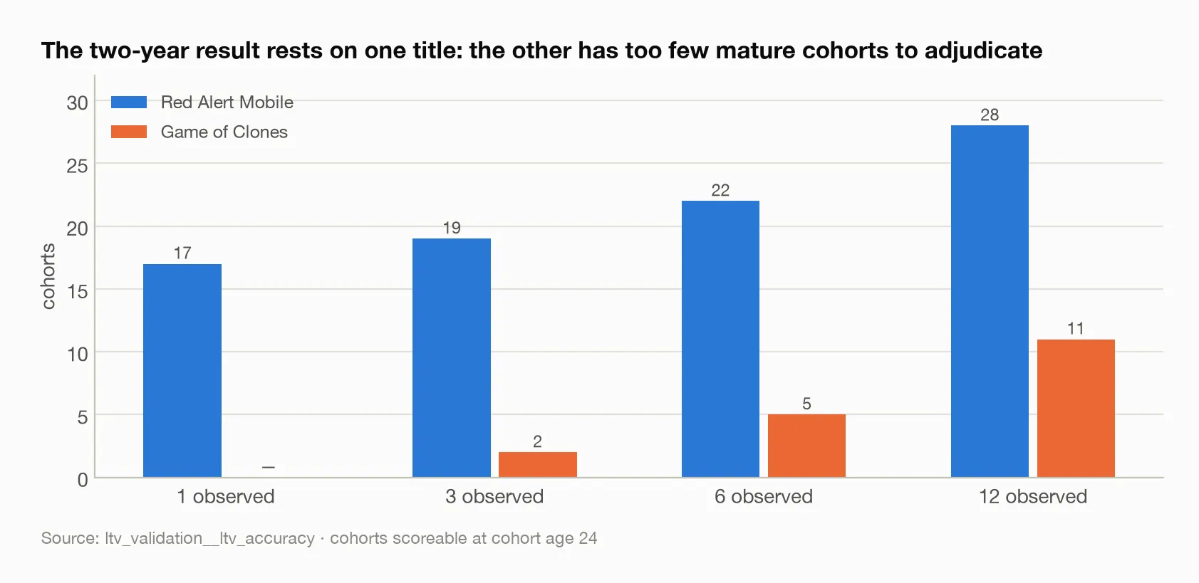
Game of Clones has no scoreable cohorts at one month observed and two at three. A comparison of three models on two cohorts is not a comparison.

The forecast is scored against everything that happened. Realised revenue includes whatever live-ops and monetisation work landed in the interim. A cohort curve does not know about a promotion. Part of the error here is measuring one.

The direction of the error is not neutral. The champion over-forecasts, modestly and consistently, on both titles and at every window. An LTV forecast that runs high makes user acquisition look more affordable than it is, so the payback it implies is optimistic. That is the wrong direction to be wrong in for the decision this feeds, and a studio using it should size that in before spending against it.

What the estimates actually say

LTV at cohort age twelve. From one, three and six months observed, the fitted curve scores 0.186, 0.146 and 0.087 on Red Alert Mobile and 0.330, 0.245 and 0.127 on Game of Clones; the ratio heuristic 0.202, 0.155 and 0.084 and 0.414, 0.214 and 0.115; banked-to-date 0.590, 0.372 and 0.200 and 0.548, 0.353 and 0.196 (ltv_validation__ltv_accuracy).

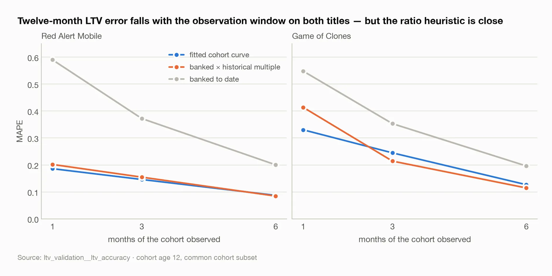
All three lines fall on both panels. The blue and orange lines are nearly on top of each other on Red Alert Mobile and cross on Game of Clones: the fitted curve wins at one month and the ratio heuristic wins from three.

Error falls monotonically with the observation window, on both titles. That is the synthetic study’s headline result, and it replicates on real data. It is the single most important thing the table says. Waiting longer genuinely buys accuracy, and it buys it in a predictable way, which is what makes an early forecast usable at all.

At one month observed the champion beats banked-to-date by 3.2 times on Red Alert Mobile and 1.7 times on Game of Clones. Against the ratio heuristic the picture is much closer: the champion loses narrowly on Red Alert Mobile from three months on and loses outright on Game of Clones from three months on. A fitted cohort curve is not a large improvement on multiplying banked revenue by a historical multiple. That is an honest result, and one worth knowing before building the more complex thing.

LTV at cohort age twenty-four, on Red Alert Mobile, where there are enough cohorts: the champion beats both baselines at every window — 0.236, 0.203, 0.131 and 0.061 from one, three, six and twelve months observed, against 0.352 to 0.075 for the ratio and 0.635 to 0.143 for banked-to-date. The Game of Clones row is unmeasured, as above.

What the synthetic benchmark said. On seeded cohorts forecasting D365 LTV (ltv_validation__ltv_synthetic_reference), the cross-cohort regression scores 0.040 from thirty days observed. Line that up against the comparable real cell — one month of a real cohort, forecasting roughly a year out — and the real champion scores 0.186 and 0.330 on the two titles: four to eight times worse.

But the more useful comparison is what happens to the baseline. Naive banked-to-date scores 0.606 on synthetic and 0.548 to 0.590 on real. The task looks about equally hard in both worlds. What collapses is how much modelling helps. On synthetic the model beats the naive baseline fifteenfold. On real data its edge is 3.2 times on one title and 1.7 on the other.

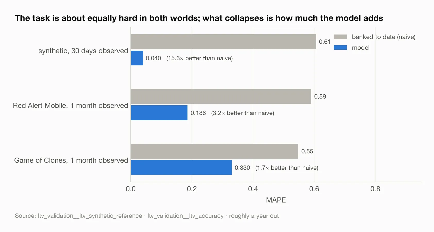
The gray bars — the naive baseline — are nearly the same height in all three rows. The blue bars are not. A synthetic benchmark overstates the model, not the problem.

That is the sharpest statement of the synthetic-benchmark problem this study produced, and it is not the one I expected. A synthetic benchmark does not necessarily overstate how easy the problem is. It overstates how much your model is adding.

Which way it is wrong. Signed bias, twelve-month LTV: the champion runs +0.197, +0.143 and +0.074 on Game of Clones and +0.098, +0.070 and +0.039 on Red Alert Mobile from one, three and six months observed. Banked-to-date under-forecasts heavily by construction; the ratio heuristic over-forecasts most of all. The champion’s over-projection has the same sign and the same growth-with-horizon as the composed revenue chain’s, which points at one shared cause rather than two.

What I would change next time

Run the LTV bake-off. The champion here is inherited from the revenue-chain work. The specification-selection grid found that the shipped default is the selected winner on none of twelve metric-account pairs. It is possible — likely, even — that a different specification does better on this task specifically.

Attribute the shared over-forecast once. The LTV forecast and the composed chain are wrong in the same direction with the same horizon profile. One cause is more likely than two, and the cohort-quality level drift is the obvious candidate.

Put the real result on a net basis. The warehouses are gross of platform fees; the synthetic generator is net. The decision a studio makes — payback on UA spend — is a net decision, and the like-for-like comparison should be too.

Wait for the second title’s cohorts to age. The two-year result is a one-title result and there is no way to hurry it.

The broader lesson

I built the synthetic generator so I could measure forecast error against a known answer, and it did that. What it could not do was tell me how much of the forecast’s accuracy came from the model and how much came from the problem being easier than a real one. The baseline is what separates those. On synthetic data the model looked like a fifteenfold improvement; on real data it is a modest improvement over a ratio a studio can compute in a spreadsheet, and on one title it is not an improvement at all past three months.

That is close to a negative result for the elaborate method, and I think it is the honest frame for when the elaborate method earns its keep: early, at one month observed, where the ratio heuristic has the least to work with, and at longer target ages on the title with enough cohorts to say. Everywhere else, a studio that multiplies banked revenue by a historical multiple is doing about as well as I did with a fitted curve — and should be told so.

The result I am most glad to have is the first one: the error falls predictably with the window, on both titles. That is the property that makes an early LTV number a decision input rather than a guess, and it is the one thing the synthetic study got right that mattered.

Sources

Every figure above traces to one of these tables:

• ltv_validation__ltv_accuracy — MAPE, bias and cohort counts by title, model, target age and observation window
• ltv_validation__ltv_synthetic_reference — the same task on seeded cohorts

forecastingltvcohort analysissynthetic datavalidation